[Intro to Computational Thinking] Introduction to Computational Thinking via Simulation with R

Example 1: Simple A/B Test Discrete probabilities

Imagine that we want to run an A/B test–randomised control trial–to evaluate the causal effect of a new treatment relative to the status quo control counterfactual. We are interested in the effect of the treatment on whether or not individuals in the study do some action–e.g. vote in an election.¹ Imagine the outcome is a discrete variable coded \([0, 1]\). Can we use a difference of means test to estimate the treatment effect?

Let’s start by hypothesizing what the data generating process could be. Imagine that based on prior research we know that there is a baseline probability of the outcome being \(1\) when a person is exposed to the control of 0.1, i.e.:

\[Y \sim \mathrm{Binomial}(0.1)\] To simulate one draw from this binomial distribution in R use:

control_y_1 <- rbinom(n = 1, size = 1, prob = 0.1)
control_y_1

## [1] 0

Let’s walk through this code. rbinom() is the function to randomly (the r in rbinom) draw from the binomial distribution (binom). n is the number of draws for this simulation, size is the “number of trials”. Basically it means that you want the “success” outcome to be 1 and 0 otherwise. prob is the probability of “success”.

It’s unlikely that we will run an A/B test with only one participant in the control group (this would be hilariously under-powered). So, let’s simulate a test with 2,000,000 draws² and plot the results.

# number of observations variable to ensure consistency across sims
n_obs <- 2e6
control_prob <- 0.1

control_y <- rbinom(n = n_obs, size = 1, prob = control_prob)
hist(control_y)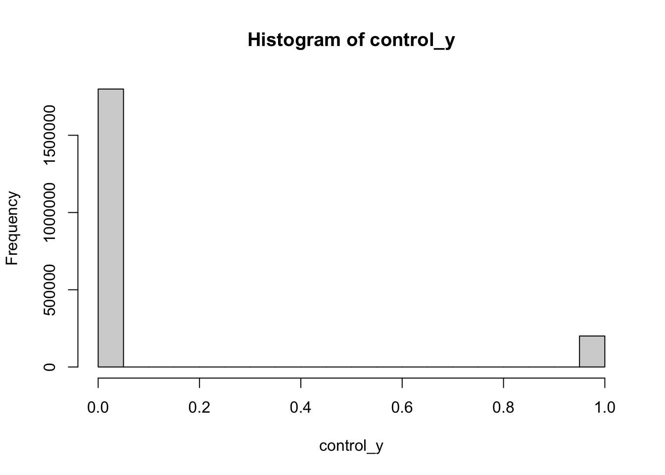

Side note: Histograms with ggplot2

ggplot2 is a very powerful way to create graphics in R. Here is an example of how you would create a histogram with ggplot2.

# ggplot2 is a member of the "tidyverse" set of packages
xfun::pkg_attach2("tidyverse")

# I personally enjoy the simplicity of the "linedraw" theme
theme_set(theme_linedraw())

# ggplot cannot accept a vector, like `hist` 
# You need to convert to a data frame or the tidyverse equivalent "tibble"
control_y_tbl <- as_tibble(control_y)

# Plot and change the x-axis label
ggplot(control_y_tbl, aes(x = value)) + # as_tibble names the column "value" by default
  geom_histogram() + 
  xlab("\nControl Outcome") + # \n adds a line break before the label
  ggtitle("Simple Simulation Histogram", subtitle = "Control Group")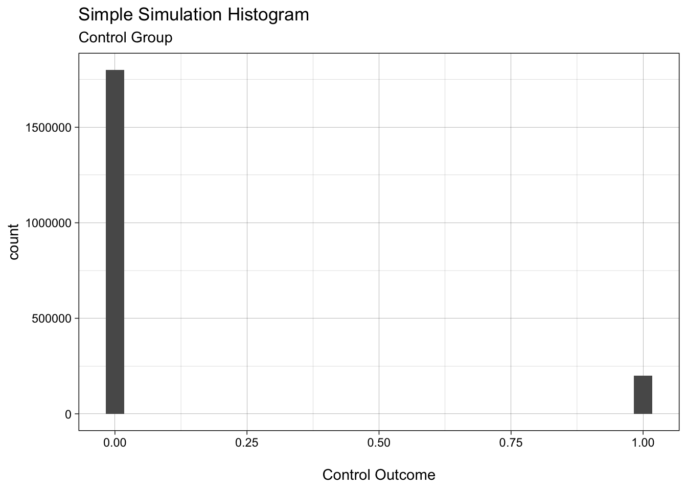

Notice how you build up the layers of the plot in ggplot by adding “geoms” with plus (+) notation. These are literally stacked on top of each other in the order you enter them in code. So the base layer is set with ggplot. This specifies the data frame to work with and the aesthetics (aes) layer that defines things like the X and Y coordinates, and grouping variables. Histograms only need the x-axis specified in aes because the y-axis will be the automatically generated count per histogram bin. But for other geoms, such as geom_point for scatter plots, you also need to specify a variable that defines the y-axis with the y argument.

If you plan to make similar ggplot plots multiple times, consider wrapping it in a function. For example:

# @param outcomes numeric vector
# @param subtitle character string of the plot's subtitle

plot_histogram <- function(outcomes, subtitle) {
  if (missing(subtitle)) stop("subtitle must be specified")
  x_tbl <- as_tibble(outcomes)
  ggplot(x_tbl, aes(x = value)) + 
  geom_histogram() + 
  xlab("\nControl Outcome") +
  ggtitle("Simple Simulation Histogram", subtitle = subtitle)
}

plot_histogram(outcomes = control_y, subtitle = "Control Group")

Ok, we’ve simulated one run of the control group. Now let’s think about the treatment group. Imagine we anticipate that a realistic effect of the treatment–again based on prior knowledge–is an average relative improvement of 1%. We simulate this with:

rel_effect <- 0.01
treat_prob <- control_prob + (control_prob * rel_effect)
treatment_y <- rbinom(n = n_obs, size = 1, prob = treat_prob)

plot_histogram(treatment_y, subtitle = "Treatment Group")

Finally, we compare the means of the two groups:

mean(treatment_y) - mean(control_y) 

## [1] 0.0006515

That’s one simulation. Let’s wrap it up in a function so it will be easy to run \(n\) simulations

# @param n integer number of draws per treatment arm
# @param control_prob numeric probability of control success [0, 1]
# @param rel_effect numeric relative effect, change in success probability 
# caused by treatment 

one_sim <- function(n, control_prob, rel_effect) {
  treat_prob <- control_prob + (control_prob * rel_effect)
    
  cy <- rbinom(n = n, size = 1, prob = control_prob)
  ty <- rbinom(n = n, size = 1, prob = treat_prob)
  
  mean(ty) - mean(cy)
}

Let’s test it to make sure it works.

one_sim(n = n_obs, control_prob = control_prob, 
        rel_effect = rel_effect)

## [1] 0.0005305

This is very close to the true increase absolute of 0.001 (i.e. 1% of the control_prob of 0.1).

Monte Carlo with for

Now that we’ve created a function for one total draw of the simulated A/B test, let’s repeatedly sample it so that we can better understand the probabilistic properties of our hypothesized data generating process.

One way to do this is with for loops. For example:

# package to add a progress bar to monitor loop progress
xfun::pkg_attach2("progress")

# Create vector of NAs to take the simulation results
n_sims <- 100
mean_diff <- rep(NA, n_sims)
pb <- progress_bar$new(total = n_sims)

for (i in seq_along(mean_diff)) {
  pb$tick() # increment the progress bar
  mean_diff[i] <- one_sim(n = n_obs, control_prob = control_prob, 
        rel_effect = rel_effect)
  #if (is.na(mean_diff[i])) stop(paste(i, "is missing"))
}

hist(mean_diff)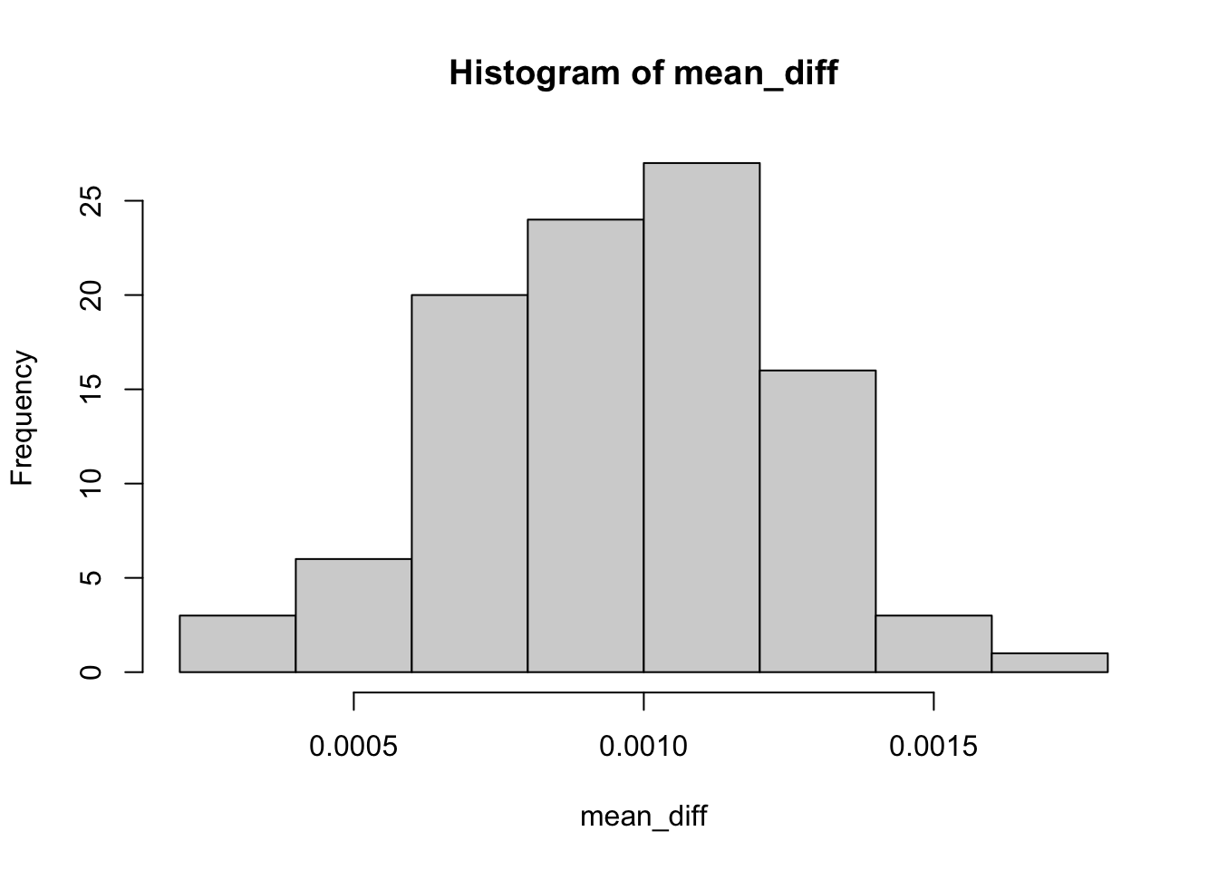

Monte Carlo with apply and parallelization

for loops are notoriously slow in R.⁴ This isn’t a problem if you are only doing a few simulations, but gets very tedious if you need to run many simulations. Often–though not always–using the apply family of functions is faster. They also can make it easier to parallelize your code.

Since we want to run the same function n times, we can use the replicate() helper function for the apply family:⁵

system.time(
  mean_diff <- replicate(n_sims, one_sim(n = n_obs, 
                                       control_prob = control_prob, 
                                       rel_effect = rel_effect))
)

##    user  system elapsed 
##   5.695   0.135   5.834

I wrapped this call in system.time() so that we can keep track of how much computation time we spend on the call. Monte Carlo simulations are just doing the same thing over and over. This computation time can add up.

We can see that the the apply version (above) in this case is pretty much as slow as the for loop (below).⁶

system.time(
  for (i in seq_along(mean_diff)) {
    mean_diff[i] <- one_sim(n = n_obs, control_prob = control_prob, 
        rel_effect = rel_effect)
  }
)

##    user  system elapsed 
##   5.682   0.140   5.826

So far we have been running all of our simulations in sequence. However, each simulation, by construction, is independent of the others. This is a perfect use case for parallelization.

There is a mc_replicate() helper function (originally from the rethinking package) that makes this easy for the code we have written so far.

xfun::pkg_attach2("mcreplicate")

system.time(
  mc_replicate(n_sims, one_sim(n = n_obs, 
                              control_prob = control_prob, 
                              rel_effect = rel_effect),
              mc.cores = 4)
)

##    user  system elapsed 
##   4.681   0.159   1.660

As we would expect from running the simulations across 4 rather than one core, the elapsed time is faster with mc_replicate(). Note it is not 4 times faster in this case, because there is overhead in setting up the parallelization. With more samples we the overhead as a proportion of total computation time will decrease and we will approach 4x computation time.

Finally, let’s see if the difference of means is a useful way of estimating the treatment effect for a binary outcome? Let’s run a few more simulations. We should see normally distributed difference of means centered on 0.001:

diff_means_1000 <- mc_replicate(1e3, one_sim(n = n_obs, 
                                      control_prob = control_prob, 
                                      rel_effect = rel_effect),
                              mc.cores = 4)

# find mean of all simulations for plotting
mean_of_means <- mean(diff_means_1000)

# plot simulations with line at mean value
diff_means_1000_tbl <- as_tibble(diff_means_1000)

ggplot(diff_means_1000_tbl, aes(value)) +
  geom_histogram(alpha = 0.6, fill = "#29ffc6") +
  geom_vline(xintercept = mean_of_means, linetype = "dashed") +
  xlab("\nTreatment - Control") +
  ggtitle("Monte Carlo Results", 
          subtitle = "Difference of means for binary outcome\n1,000 simulations")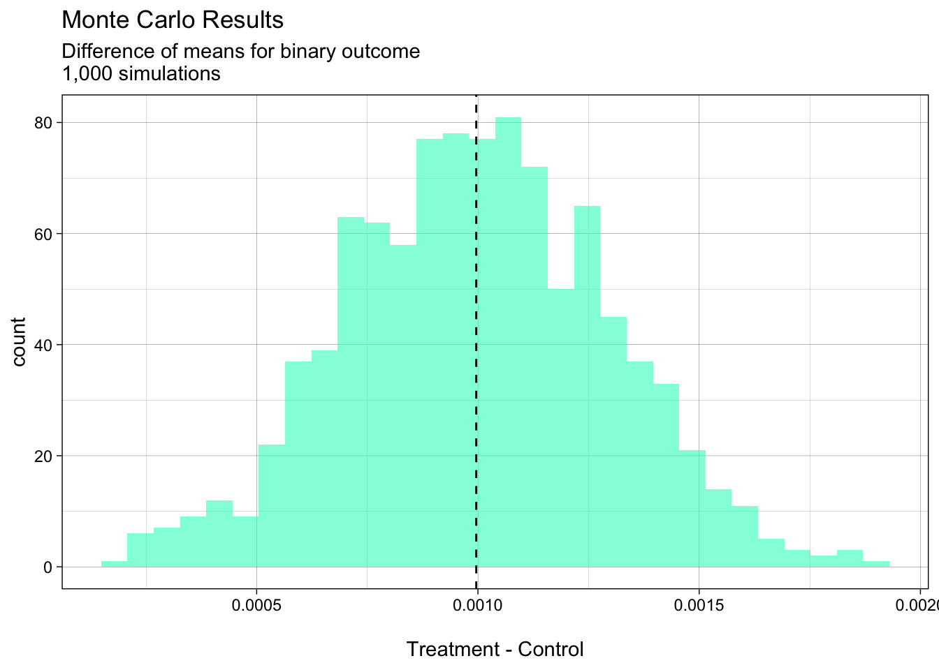

In this example, the more simulations we run, the more smooth and “normal” the curve will become.

Being mindful of your feelings

We’ll cover the the technical debugging tools available in R. But I first want to first mention a crucial part of effective (and less stressful) debugging: being mindful of your feelings about the bug.

A bug is frustrating. Our first encounter with a bug is an experience of disassociation between how we think the world should work and how it is working. It’s as if we want to put a plate in the cupboard, but each time we try to put the plate in the cupboard it flies out. Frustration inclines us to look for the cause of a bug in–almost always–the wrong place: “the stupid computer is broken”.

The best way to resolve bugs, as we’ll see, is to create testable hypotheses about what could be causing the bug. “The stupid computer is broken” is vague and so not a testable hypothesis.

So, it is crucial that when you find a bug, to take a step back and ask:

how does this bug make me feel?

If the answer is “angry, I want to throw my computer out the window”, your best next step is to take a break. Grab a tea or whatever. Then, with a piece of paper (or some other tool that gets you away from the temptation to just begin slamming out code on your keyboard) write down hypotheses about the cause of the bug and ways to test them.

Unlike social phenomena, many computer bugs are deterministic. The cause of a bug will usually cause the bug. So your chances of definitively finding the bug are high with the following process and tools.

Clear and testable program specifications

Finding your bug is a process of confirming the many things that you believe are true — until you find one which is not true.

—Norm Matloff (quote from Advanced R)

Great debugging is driven by having great expectations of what the program should return. Having a well defined expectation of what a program should do is important to knowing if you have a bug to begin with. One way to approach software development is to write tests for a function before you write the function. This is called test driven development.

Both in your functions, to test incremental expectations, and for the output of your functions you include automated tests. Here is a silly example. Imagine that we have a function that should add 2 + 2 and then divide by 2 to return 2. We can create an automated test like this:

# Function to test
two <- function() {
  four <- 2 + 2
  if (four != 4) 
    stop("Did not add 2 + 2 correctly")
  
  four / 2
}

# Automated test 
if (two() != 2) stop("function two did not return two")

The if . . . stop statements automatically test whether or not the function is executing correctly. If there is a problem, the tests should help us pinpoint the cause more quickly.

Automated tests will also help us make sure that our code is correct even as we change it, for example, to add new features.

browser() for testing and dissecting

A key debugging R tool is the browser() function. When R executes some code and hits browser() it stops the execution and begins an interactive Browse mode. This allows you to explore objects created in the code execution in the environment that created then, as well as run new code. RStudio works really well with this function.

Imagine we wrote the loop above incorrectly:

one_sim_bug <- function(n, control_prob, rel_effect) {
  treat_prob <- control_prob / (control_prob * rel_effect)
    
  cy <- rbinom(n = n, size = 1, prob = control_prob)
  ty <- rbinom(n = n, size = 1, prob = treat_prob)
  
  mean(ty) - mean(cy)
}

mean_diff_bug <- rep(NA, n_sims)

for (i in seq_along(mean_diff)) {
  mean_diff_bug[u] <- one_sim_bug(n = n_obs, 
                                  control_prob = control_prob, 
                                  rel_effect = rel_effect)
}

We have two layers of nested functions where the bug could be. Let’s systematically use browser() to identify the source. Start from the outer most function–the for loop and work you way down as necessary.

for (i in seq_along(mean_diff)) {
browser()
  mean_diff_bug[u] <- one_sim_bug(n = n_obs, 
                                  control_prob = control_prob, 
                                  rel_effect = rel_effect)
}

Ok, we’ve found the typo. We should have used i instead of u to index the output of one_sim. To leave the browser environment type c + Enter (or on some Windows machines Q + Enter). Are we done? We’ll let’s check the output:

for (i in seq_along(mean_diff)) {
  mean_diff_bug[i] <- one_sim_bug(n = n_obs, 
                                  control_prob = control_prob, 
                                  rel_effect = rel_effect)
}

hist(mean_diff_bug)

Hm, we are not getting a valid histogram. Let’s now go down the function nesting to insert a browser() call in one_sim:

one_sim_bug <- function(n, control_prob, rel_effect) {
  browser()
  treat_prob <- control_prob / (control_prob * rel_effect)
    
  cy <- rbinom(n = n, size = 1, prob = control_prob)
  ty <- rbinom(n = n, size = 1, prob = treat_prob)
  
  mean(ty) - mean(cy)
}

mean_diff_bug <- rep(NA, n_sims)

for (i in seq_along(mean_diff)) {
  mean_diff_bug[u] <- one_sim_bug(n = n_obs, 
                                  control_prob = control_prob, 
                                  rel_effect = rel_effect)
}

When we do this, we can find that we incorrectly divide control_prob by (control_prob * rel_effect) the ultimate result, is that the output of one_sim is NA. We can’t create a histogram of NAs. Once we solve this issue, we should get the expected histogram.